Step 1: Create a new Project folder by clicking ![]() . Enter a Title and Description (both can be edited at a later time).
. Enter a Title and Description (both can be edited at a later time).
Step 2: Select "Partner Recommended Analysis" to access NanoString assay workflows, then click Next.
Step 3: Select "NanoString nCounter Data Analysis"

Then click Next.
Step 4: Select "Gene Expression nCounter RCC".

Then click Next.
Step 5: Enter an "Experiment Title" and "Description" (both can be edited at a later time)
Then click Next.
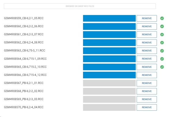
Step 6: Click the "Browse or
Drop RCC Files" upload box to navigate to and select the demo RCC files for upload, or drag and drop into the upload box to begin upload*.
Files will immediately begin uploading. Once all sample files have been uploaded, a green checkmark will appear next to the file.
Click Next .
*If analyzing your own data, select your own RCC files for upload
Step 7: ROSALIND intelligently auto-detects the species and panel of your files, but if your samples are of a different species or a different panel you can select the correct species and panel from the dropdown menu.
Demo files are Human (Homo Sapien) CAR-T Characterization panel.
Click Next.
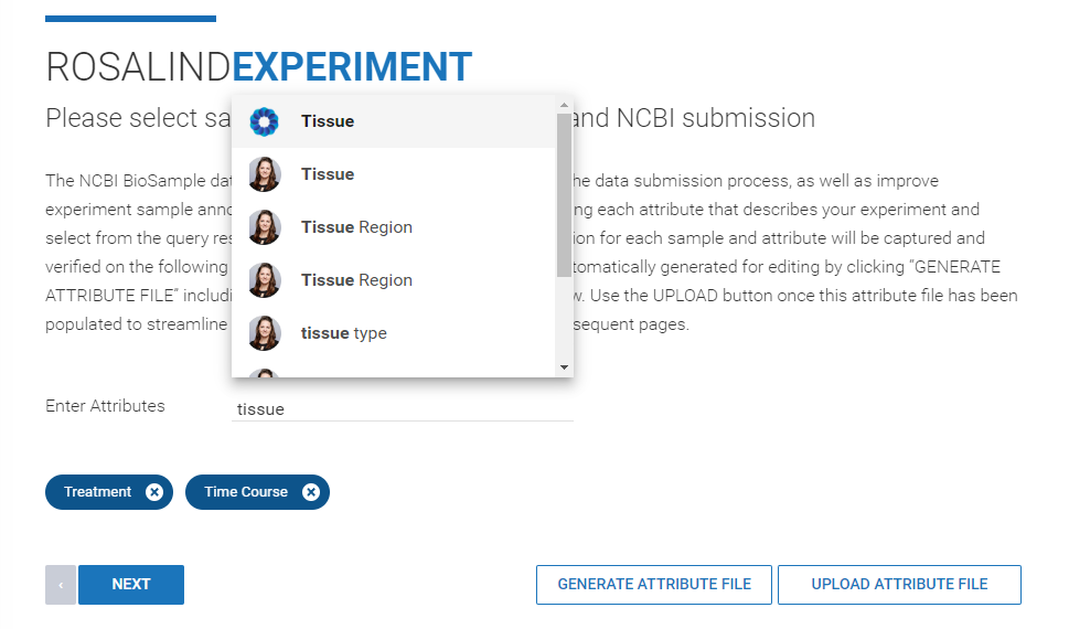
Step 1: Specify sample attributes by typing the attribute categories into the "Enter Attributes" line.
Enter the following attributes: "Source Name" and "Treatment"
Learn:
To learn how to create your own attribute file, download the blank experiment attribute file (.CSV format) by clicking ![]() .
.
NanoString attribute files will auto generate the first column as "Sample Name", which will match the uploaded RCC file names. Do not change this column. Use the Sample Replacement column to enter a unique sample name for each sample that will be used in QC and results representations.
Within the attribute csv file, attribute values can be manually assigned to each sample.
*If uploading your own data, create an attribute file for your experiment and upload in the next step.
Step 2: Upload the demo attribute file* into ROSALIND by clicking ![]() .
.
Click Next.
Step 3: ROSALIND provides a sample sheet to review for accuracy of sample information, changes can be made directly on the sample sheet if needed.
Once reviewed, click ![]() .
.
Learn:
Learn about nCounter Advanced features options and which journey is best for your data.
Step 1: ROSALIND will immediately begin initializing and processing the data in preparation for pruning and normalization (Note: this may take up to several minutes depending on the size of the data).
Once finalized, an option between Default and Advanced (available to paid subscribers) options will become available.
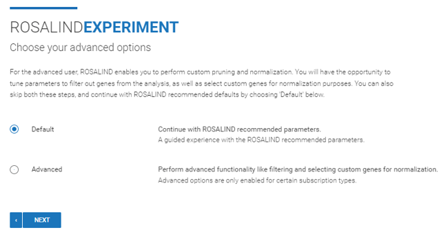
Default: This option is available to all users. Default parameters for probe pruning and housekeeper selection will be applied. To learn more, see the nCounter Methods section in Knowledge Hub.
If this option is selected, proceed to Chapter 4.
Advanced: *This option is available to ROSALIND Paid Subscribers. Select this option for custom probe pruning and selection of probes for normalization.
Step 2 (Advanced): Thresholds and probes for pruning can be customized. Default parameters include Low Count Threshold, or Limit of Detection, and Sample Frequency Default.
Low Count Threshold is a unique value to your dataset calculated from the negative probes independently across all samples to estimate the background noise of your data. If this threshold is adjusted, it will override sample-specific defaults and apply the new threshold across all samples.
Sample Frequency determines how many samples the raw expression must fall below threshold in order to be pruned. This default is set to 85%, so probes must fall below threshold in 85% of samples to be pruned.
Decreasing sample frequency is more stringent, while increasing sample frequency is more permissive.
Probes that fail both thresholds will be highlighted red, set to be pruned (removed) from the dataset, and listed in the table to the right with ![]() red arrows. Columns can be sorted by selecting the header.
red arrows. Columns can be sorted by selecting the header.

To maintain a probe in the dataset and prevent it from pruning, select the ![]() arrow next to the probe to change it to a
arrow next to the probe to change it to a ![]() blue arrow.
blue arrow.
To prune (remove) a probe from the dataset, select the ![]() blue arrow to change it to a
blue arrow to change it to a ![]() red arrow.
red arrow.

(Optional): Select ![]() to perform custom pruning outside of ROSALIND.
to perform custom pruning outside of ROSALIND.
Click, Next.
Step 3 (Advanced): Average probe expression and %CV thresholds to determine probes for normalization can be customized.
Default parameters will show an average expression of raw counts across all samples and %CV will be calculated as (standard deviation /arithmetic mean) x 100. Both thresholds can be edited by the respective sliders or by manually typing.
Housekeeping genes that pass both filters will be highlighted green, set to be included in normalization, and listed in the table to the right with ![]() red arrows. Columns can be sorted by selecting the header.
red arrows. Columns can be sorted by selecting the header.

To deselect a probe used for normalization, select the ![]() arrow next to the probe to change it to a
arrow next to the probe to change it to a ![]() blue arrow.
blue arrow.
To select a probe to use for normalization, select the ![]() blue arrow to change it to a
blue arrow to change it to a ![]() red arrow.
red arrow.

(Optional): Select ![]() to perform custom normalization outside of ROSALIND.
to perform custom normalization outside of ROSALIND.
Click, Next.
Learn:
Learn how to create comparisons and covariate correction.
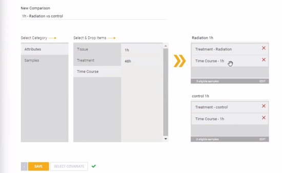
Comparisons can be configured now, prior to launching the analysis, or after the experiment has been processed and QC has been reviewed. To create a new comparison now, click ![]() . Comparisons can be created at the replicate group level (using the attributes) or individual sample level (using the sample names) by dragging and dropping different attributes or samples into the condition and control boxes on the right side of the page. Combinations of two or more different attributes can be used to create comparisons with specific subsets of samples. In the example image below, a comparison is set up across two treatment groups (Radiation vs Control) at a specific time point (1 hour). Alternatively, the comparison could be set up specifically at only the 48 hour time point, or including both time points simultaneously.
. Comparisons can be created at the replicate group level (using the attributes) or individual sample level (using the sample names) by dragging and dropping different attributes or samples into the condition and control boxes on the right side of the page. Combinations of two or more different attributes can be used to create comparisons with specific subsets of samples. In the example image below, a comparison is set up across two treatment groups (Radiation vs Control) at a specific time point (1 hour). Alternatively, the comparison could be set up specifically at only the 48 hour time point, or including both time points simultaneously.
Additionally, covariate correction can be added to the statistical model using the "SELECT COVARIATE" button. See this article to learn more about covariate correction methods.
Click the ![]() button to save the created comparison.
button to save the created comparison.
Demo Challenge:

Try creating the below comparisons with the demo data (or if using your own data, try creating a variety of comparisons as your study allows):
1) Condition vs Control:
Peripheral blood vs Cord blood
2) Condition vs Control with two attributes each:
IL2- Peripheral blood vs Cord blood
*Note: If comparisons are set up correctly, ROSALIND Intelligence will automatically name the comparison as shown in the image.
Once all comparisons have been saved, click Next.
Do not close or navigate away from the page until import is complete.

After successful import, the experiment will automatically launch. ROSALIND will notify you via email once the processing is complete and your experiment is ready for exploration.
Step 1: Navigate to and select the project folder containing the created "CAR-T Demo nCounter" experiment*. Then click into the experiment.
*If your own data was used, click into your applicable experiment
Step 2: Explore the experiment summary tab (page icon, default) ![]() for the experiment.
for the experiment.

Identify the location of the
1) Experiment title
2) Experiment description
3) Experiment setup parameters
4) Methods and citations
5) Tabs for QC exploration
Step 1: Select the Quality Control tab at the top (table icon) ![]() to navigate to the Quality Control Page.
to navigate to the Quality Control Page.
Step 2: Explore the Quality Control metrics for the experiment:
Demo Challenge:
Determine the QC of your experiment by using the table metrics:
1) Hover over each column header to learn more about each metric
2) Determine if any values are flagged
3) Determine if any samples pass or fail QC

Step 3: Click on the Sample Correlation heatmap to open the QC figure in a larger window.
Evaluate the correlation of your sample correlations in relationship to defined attributes.
Use the ![]() and
and ![]() options to further explore the plot options.
options to further explore the plot options.
Use these features to further explore each plot.

Step 4: Click on the Violin plot. Select the "Additional Images & Videos" section on the bottom left to learn more about how to interpret this plot.

Step 5: Click on the NanoString Control plot. Select "Additional Images & Videos" to visualize additional control and housekeeper data.

Step 6: Click on the Variance of mean plot and determine if housekeepers were excluded to determine which probes were used for normalization. Select the CSV download option to further explore this list.

Step 7: Click on the MDS plot and determine sample similarity between defined attributes.

Step 8: Click on the Cell Type Profiler heatmap to explore sample clustering of cell type profiles (if applicable to NanoString panel used).
Step 1: Select the Samples tab at the top (test tube icon) ![]() to navigate to the Samples Page.
to navigate to the Samples Page.
Step 2: Explore the Samples page.
Demo Challenge:
Locate the following options on your page:
1) Verify all attribute information is recorded in the table
2) ![]() to add additional attributes for differential analysis post processing
to add additional attributes for differential analysis post processing
*Note: This option is only available to the owner of the experiment
Step 1: Select the File Management tab at the top (Cloud icon) ![]() to navigate to the File Management Page.
to navigate to the File Management Page.
Step 2: Explore the different file options for download. Examples include:
1) Source Files (RCC)
2) Attribute file
3) Processed counts files
4) Differential expression results files
Step 1: Navigate to and select the project folder containing the CAR-T Demo nCounter experiment*. Then click into the experiment.
*If your own data was used, click into your applicable experiment
Step 2: Select the Discovery and Analysis Tab ![]() at the top.
at the top.
Step 3: Explore the Discovery and Analysis page
Locate the following items on your page:
1) How to create new comparisons with ![]()
2) How to create new meta-analysis with ![]()
3) Normalized Expression
4) Term Exploration

Step 1: Click into Normalized Expression

Step 2: Explore how to visualize data for single targets, multiple targets*, or a gene list in multiple views
*Note: To select multiple targets, hold CTRL or CMD and click targets of interest

Step 1: Click into Term Exploration to explore Cell Profiling Results

Step 2: Explore how to visualize Cell Type Profiling annotations and scores as a box plot, bar graph, heatmap, or data table.
*Note: Cell Profiling results are only available for certain off-the-shelf panels

Step 1: Click into the "Peripheral blood vs Cord blood" created differential analysis comparison

Step 2: Identify the significantly differentially expressed genes on the left-hand side and the default parameters determined by ROSALIND Intelligence.

Step 3: Explore the volcano plot interactivity.

Step 4: Toggle the sample normalized expression chart between individual samples and sample groups box plot.

Step 5: Explore the heatmap interactivity.
Custom Visualizations: To create a custom volcano plot and heat map, hold down the control key on a PC keyboard or command key on a MAC keyboard, while clicking multiple genes from the list on the left or select a pre-created gene list (see this article for more information on how to create a gene list).
Custom Tabs: The tabs on the left margin of the significant gene list allow for visualization and exploration customization. Explore each tab:
Filter tab ![]() : represented by the funnel icon, allows the option to switch between created
: represented by the funnel icon, allows the option to switch between created

filters or create new filters. Select the plus "![]() " icon to create a new filter.
" icon to create a new filter.
Within the Create a New Filter page, enter a new filter name, cut-off values, adjusted or unadjusted p-value option and optional color icon. Select ![]() to update the table on the right with applicable genes according to the filter parameters.
to update the table on the right with applicable genes according to the filter parameters.
Continue adjusting the parameters until satisfied with the gene output, then click ![]() .
.
The new filter and associated interactive analysis output will begin processing. You will receive an email to begin exploring the data when processing is complete.
Group tab ![]() : represented by three horizontal lines, allows grouping of significant genes.
: represented by three horizontal lines, allows grouping of significant genes.
Select whether to group genes by "Clusters" or "Not Grouped".

Then select how to sort the gene list.

Search tab ![]() : represented by a magnifying glass, opens a search bar that can be used for a gene or list of genes.
: represented by a magnifying glass, opens a search bar that can be used for a gene or list of genes.
Color Pallet tab ![]() : represented by a colored circle, allows customization of the heatmap color scheme.
: represented by a colored circle, allows customization of the heatmap color scheme.
Find your favorite heatmap color.
Custom Pathways: Explore the pathway table on the right.
ROSALIND Intelligence Enrichment Summary: lists the key pathways and terms that are the most representative of the important biological changes in your system from across all 50 knowledge bases.
*Note: if less than 50 significant pathways are found within your comparison, the ROSALIND Intelligence algorithm will not run and the Summary will simply display the top 50 pathways ranked by adjusted p-value.

Pathways Summary: Specific pathways can be selected from the drop-down menu from across 50 knowledgebases.

Click a pathway of interest to explore. Note how all visualizations change upon selection of a pathway to facilitate deep exploration.

Knowledgebase Deep Dive: Pathways can be visually explored on a deeper level by clicking the magnifying glass ![]() on the pathways summary page. A complete view of results for each knowledgebase can be explored by clicking on the magnifying glass on the pathway summary page.
on the pathways summary page. A complete view of results for each knowledgebase can be explored by clicking on the magnifying glass on the pathway summary page.

Explore the full results for a knowledgebase by altering its Chart Type, Sort By, and Color menu options.

To view pathway diagrams and visualizations, select the Wikipathways knowledgebase under the "List Type" drop down menu. Then click on the Gold magnifying glass ![]() for a pathway of interest to view the corresponding diagram.
for a pathway of interest to view the corresponding diagram.
To return to the interactive analysis dashboard, select the differential analysis tab ![]() at the top of the page.
at the top of the page.

Volcano Plot/Box Plot: To download the volcano plot or box plot, click on the visualization to open up a new window with options for download.
Heatmap: To download the heatmap, click on the heatmap to initiate an immediate download to your hard drive.
Lists and select views: To download lists such as filter views and pathway visualizations, select the cloud icon ![]() to initiate download.
to initiate download.
*Note: Some larger images may take longer to download. Clicking quickly or on multiple images will initiate multiple downloads which may be blocked by your browser. For more information on how to adjust these settings, see the FAQ section of this article.
Complete this 1-minute survey to receive a certificate of completion.
We would love to hear your feedback and experience taking this course.

Thank you, we appreciate your time!